PART 1: Filtering, Edges, and Gradients
1.1 Convolutions from Scratch vs. SciPy
To understand what happens under the hood during spatial filtering, I implemented 2D convolution from scratch using pure NumPy. I built two versions as required per the assignment which included a naive 4-nested-loop implementation
# Loop ONLY over kernel taps, vectorizing image slice additions
for row in range(rows):
    for col in range(cols):
        pixel_sum = 0.0
        for i in range(k_rows):
            for j in range(k_cols):
                pixel_sum += padded_image[row + i, col + j] * kernel_flipped[i, j]
        output[row, col] = pixel_sum

return output# Loop ONLY over kernel taps, vectorizing image slice additions
for k_r in range(k_rows):
for k_c in range(k_cols):
output += padded[k_r:k_r + rows, k_c:k_c + cols] * kernel_flipped[k_r, k_c]
return outputscipy.signal.convolve2d using zero-padding (mode='constant', constant_values=0).
Mathematical Definition: For an image \(I\) and kernel \(K\) of size \(k_r \times k_c\), 2D convolution flips the kernel in both axes (\(K_{\text{flipped}}[i,j] = K[k_r-1-i, k_c-1-j]\)) and computes:
\[O[r, c] = \sum_i \sum_j \text{Padded\_I}[r + i, c + j] \cdot K_{\text{flipped}}[i, j]\]
I tested the convolutions on my self-portrait (far.jpg) using a \(9 \times 9\) normalized box filter, as well as horizontal (\(D_x = [1, 0, -1]\)) and vertical (\(D_y = [1, 0, -1]^T\)) finite difference operators.
(see Figure 1a-1d below)
Performance Benchmark Results
| Implementation Method | Execution Time (s) | Speedup vs 4-Loop | Max Absolute Error vs SciPy |
|---|---|---|---|
SciPy convolve2d |
0.326632s | 164.5x faster | N/A |
| Custom 2-Loop (Vectorized Slices) | 0.940454s | 57.1x faster | 2.44e-15 (Exact Match) |
| Custom 4-Loop (Naive Nested) | 53.725185s | 1.0x (Baseline) | 2.44e-15 (Exact Match) |
Takeaway on Vectorization: Iterating over every individual pixel across 4 nested Python loops is brutally slow due to interpreter overhead (taking over 53 seconds!). By vectorizing the inner spatial dimensions and iterating only over kernel taps (2 loops), NumPy delegates array slicing to C-level loops, bringing runtime down to 0.94 seconds—a massive 57.1x speedup while achieving a great precision when compared to SciPy.
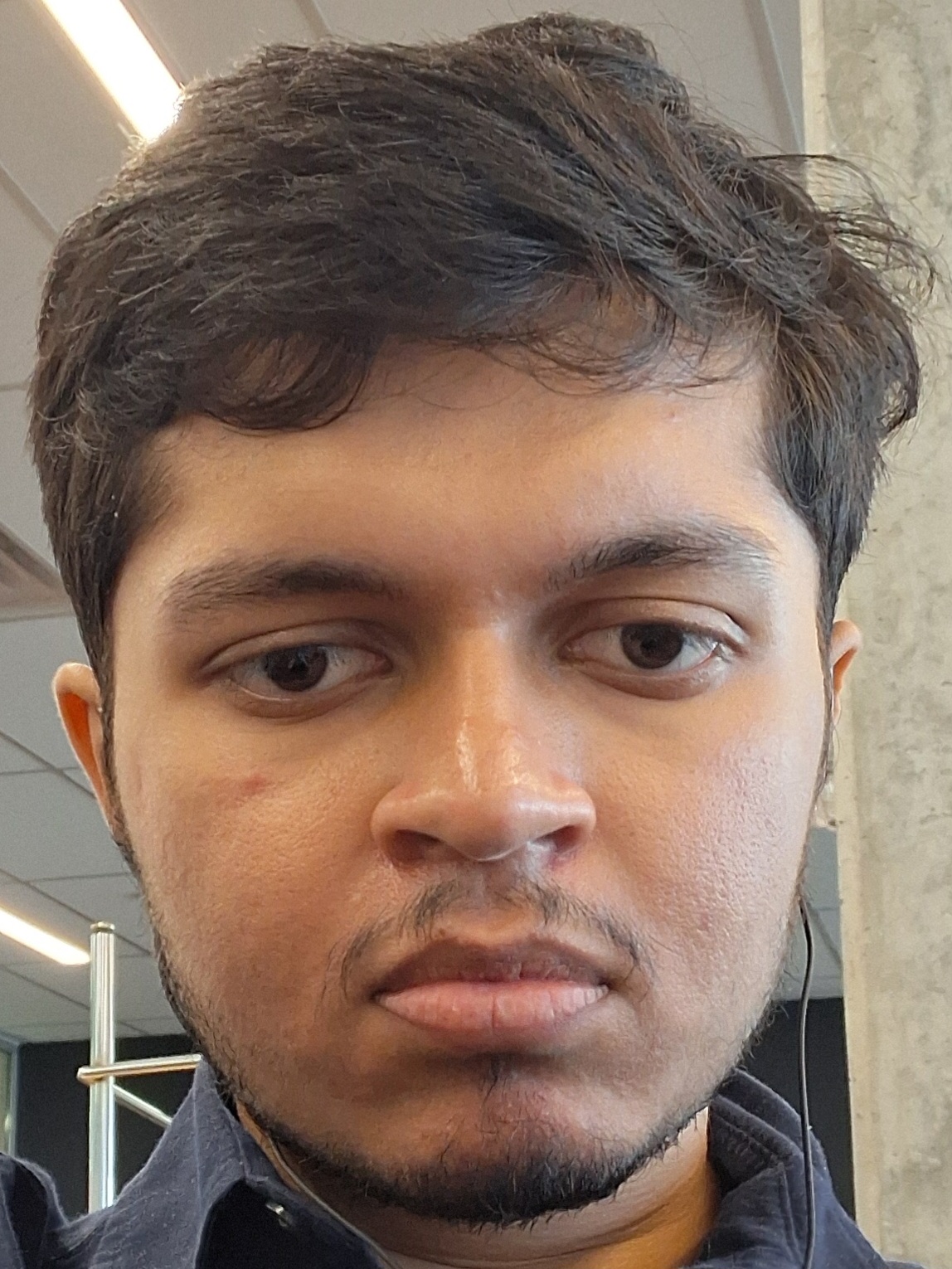
Figure 1a. Self-portrait taken using a camera
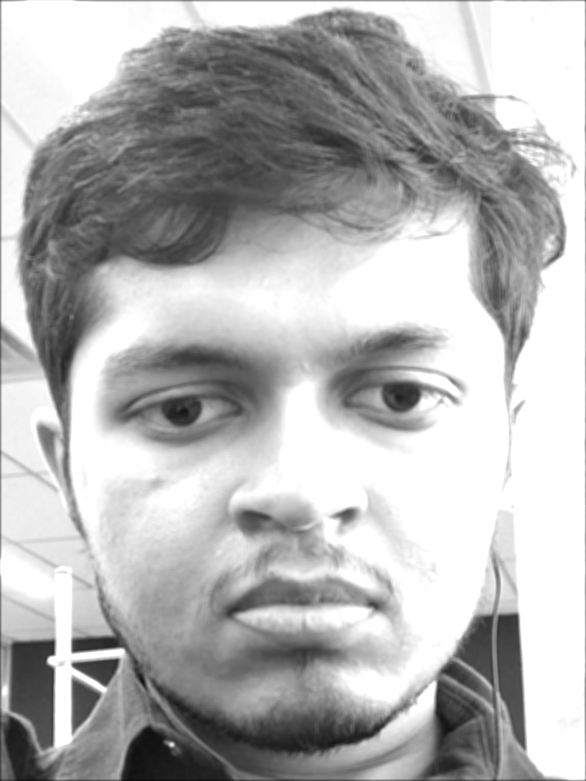
Figure 1b. Self-portrait blurred using a 9x9 box-filter
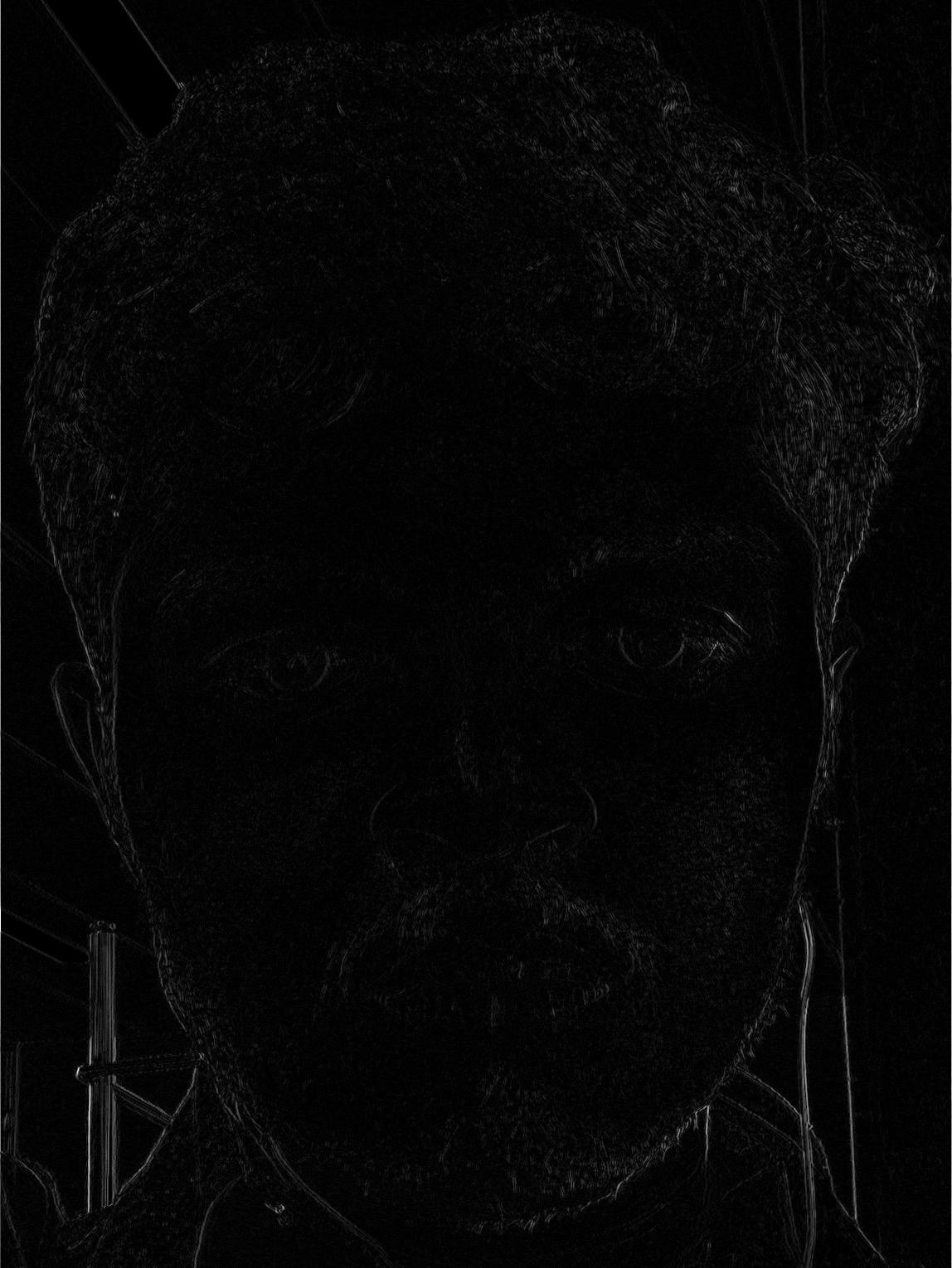
Figure 1c. Self-portrait convolved using D_x
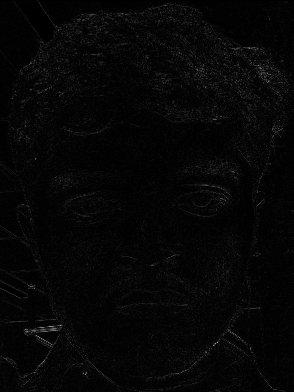
Figure 1d. Self-portrait convolved using D_y
1.2 Finite Difference Operator
Next, I applied the finite difference operators \(D_x = [1, 0, -1]\) and \(D_y = [1, 0, -1]^T\) to the classic cameraman.png image to extract partial spatial derivatives, compute the gradient magnitude image, and produce a binarized edge map.
Gradient Magnitude Formula:
\[\|\nabla I\| = \sqrt{G_x^2 + G_y^2} = \sqrt{(I * D_x)^2 + (I * D_y)^2}\]
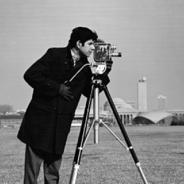
Figure 2a. Original image of Cameraman
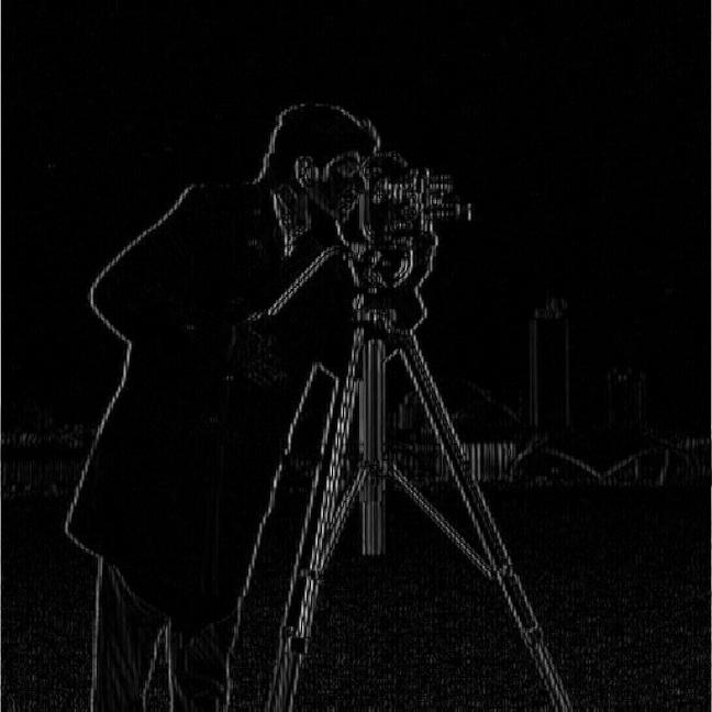
Figure 2b. Original image of Cameraman convolved using D_x
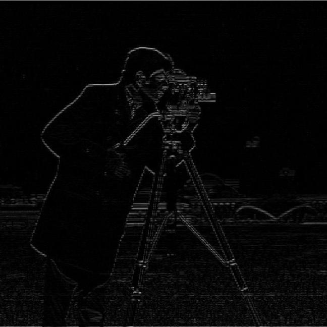
Figure 2c. Original image of Cameraman convolved using D_y
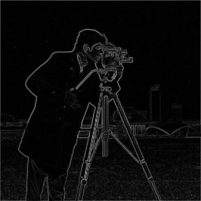
Figure 2d. Gradient Magnitude of original image of Cameraman
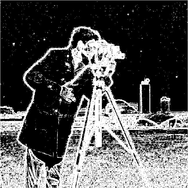
Figure 2e. Binarized Original image- Threshold = 0.025
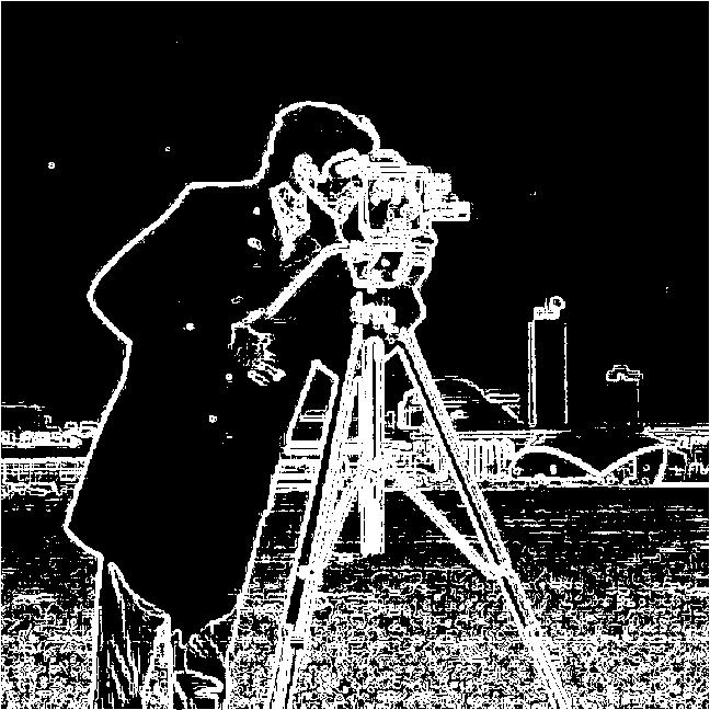
Figure 2f. Binarized Original image- Threshold = 0.050
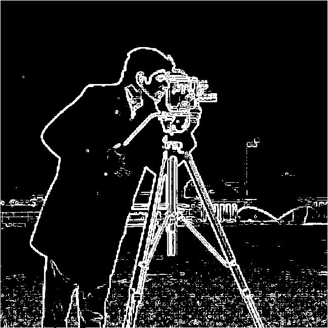
Figure 2g. Binarized Original image- Threshold = 0.100
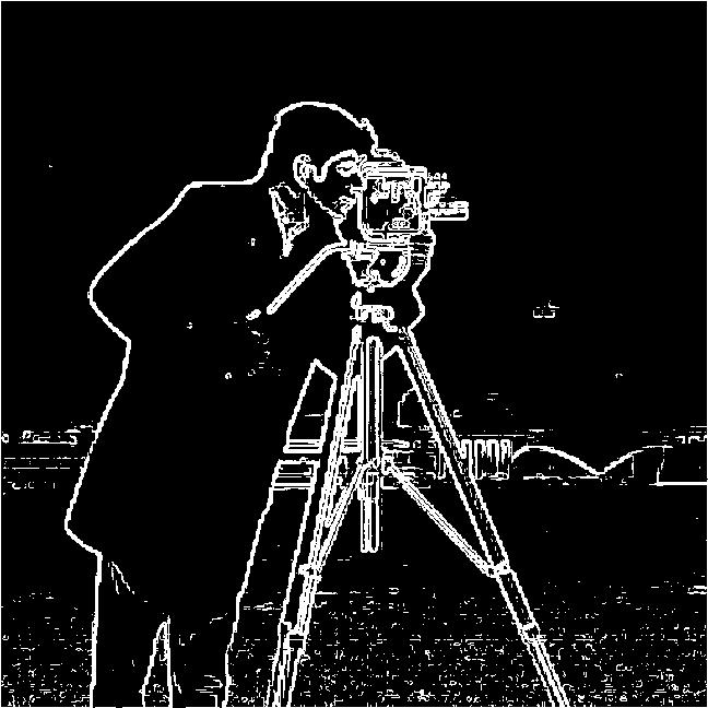
Figure 2h. Binarized Original image- Threshold = 0.125
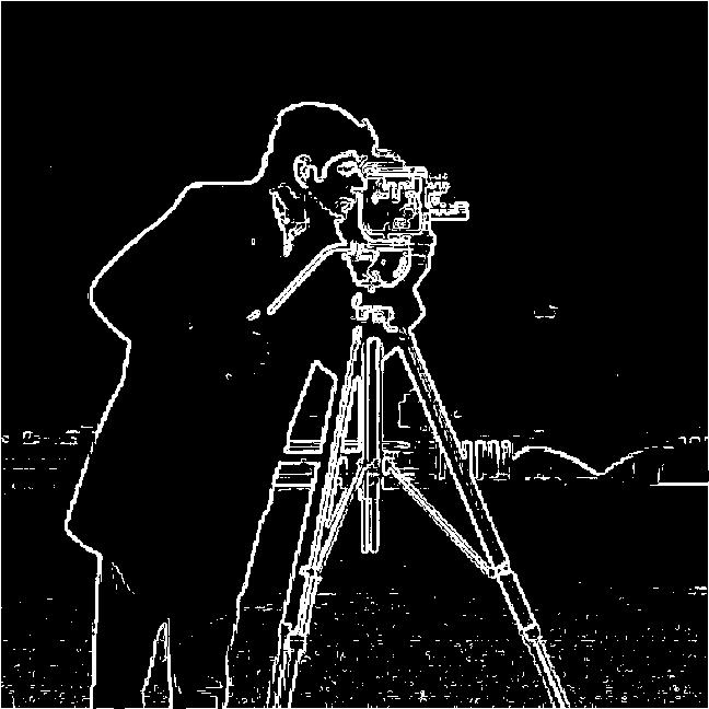
Figure 2i. Binarized Original image- Threshold = 0.150
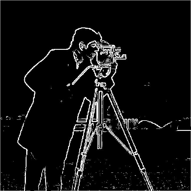
Figure 2j. Binarized Original image- Threshold = 0.175
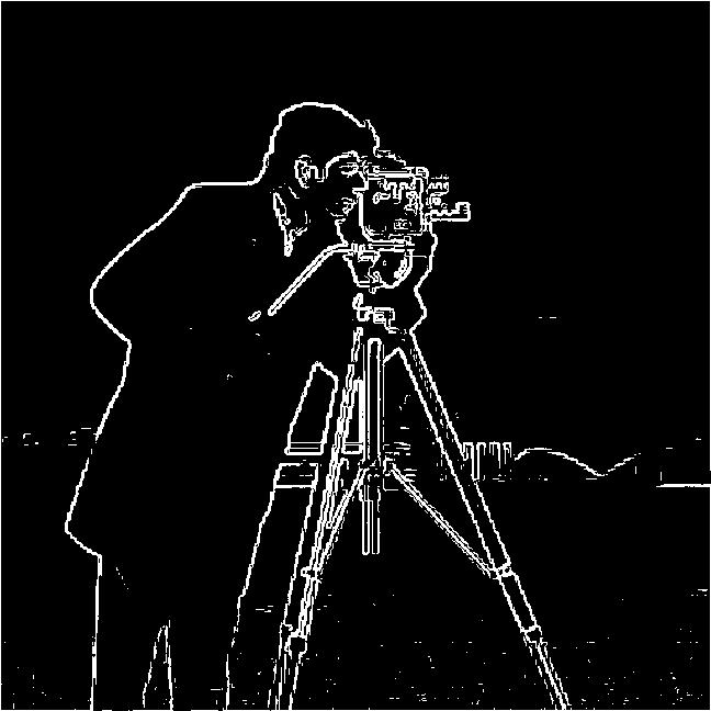
Figure 2k. Binarized Original image- Threshold = 0.200
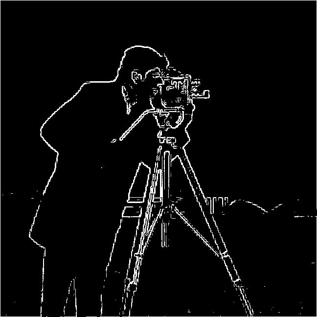
Figure 2l. Binarized Original image- Threshold = 0.250
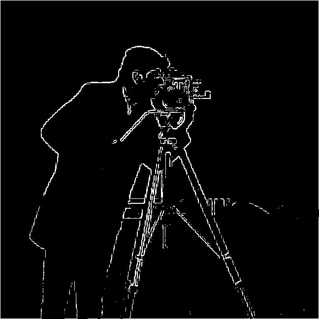
Figure 2m. Binarized Original image- Threshold = 0.300
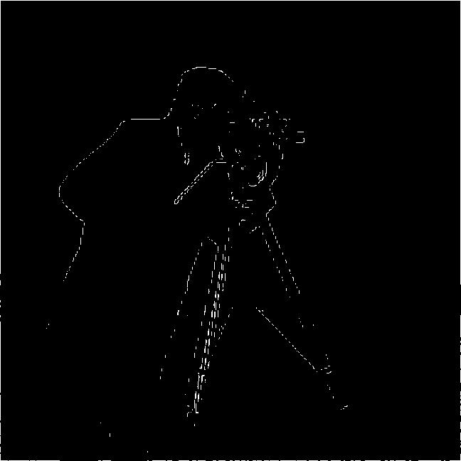
Figure 2n. Binarized Original image- Threshold = 0.500
Threshold Justification & Trade-offs: Setting a threshold when binarizing is basically setting a cut off that pixels below X value should be of either color (black or white), hence binarizing.
Selecting a threshold of 0.200 represented the sweet spot for edge extraction (you can see the Figures 2e-2n above). It cleanly captured the prominent contours of the cameraman's coat, tripod, and face while suppressing high-frequency grass noise in the foreground. The tradeoff was to let the background building tower faint outline disappeared (you can observe it being disappeared from when threshold was 0.050 and as it was gradually increased to 0.200 where it almost completely disappears). If I lowered the threshold below 0.125 to bring back the background tower, the grass foreground exploded into a noisy clutter of false-positive edge pixels which would made it harder to recognize the facial features of the cameraman. So in short, the cameraman was the subject and thats what I wanted to focus on more.
1.3 Derivative of Gaussian (DoG) Filter
Raw finite differences are extremely sensitive to high-frequency sensor noise. To solve this, I smoothed the image with a 2D Gaussian filter (\(k=5, \sigma=1\)) before taking derivatives. I also verified the single-pass DoG trick by pre-convolving the Gaussian kernel with \(D_x\) and \(D_y\) (\(DoG_x = G * D_x, DoG_y = G * D_y\)).
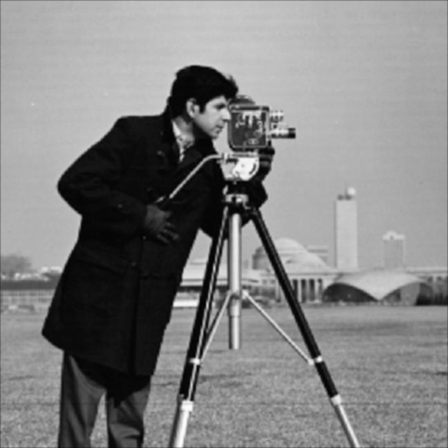
Figure 3a. Gaussian smoothed image
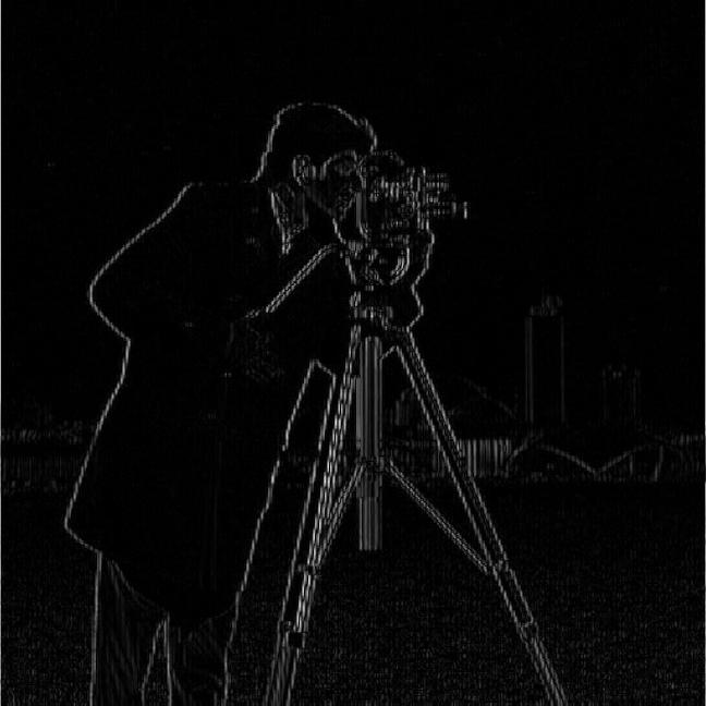
Figure 3b. DoG_x Filter Kernel (G * D_x)
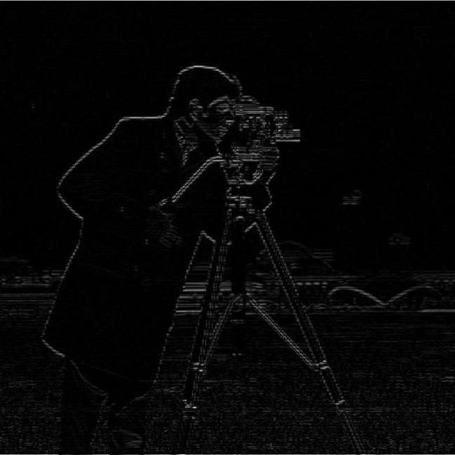
Figure 3c. DoG_y Filter Kernel (G * D_y)
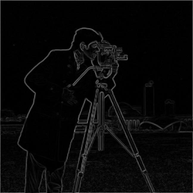
Figure 3d. DoG Gradient Magnitude
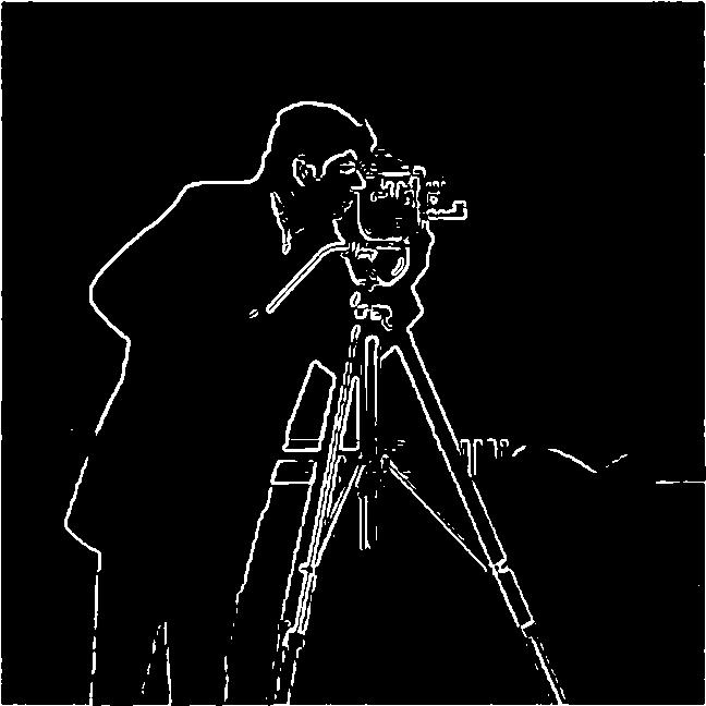
Figure 3e. DoG Binarized Edge Map with threshold = 0.200
Observations & Comparison vs Part 1.2: The DoG gradient magnitude map is dramatically cleaner and smoother
Figure 3d. DoG Gradient Magnitude
Figure 2d. Gradient Magnitude of original image of Cameraman
Figure 3e. DoG Binarized Edge Map with threshold = 0.200
Figure 2k. Binarized Original image with no DoG- Threshold = 0.200
Bells and Whistles (Part 1): Gradient Orientations
For this part I had to find the direction of the gradient at every pixel as a full angle from 0 to 2\(\pi\), without calling np.arctan2 or math.atan2. So I wrote my own (with the help of references below in References section). The idea is to shrink the problem to one small, easy case, approximate that case with a short polynomial, and then undo the shrinking so the angle lands in the right place.
The first step is to make the problem small. I take the absolute values of \(G_x\) and \(G_y\) and divide the smaller by the larger, which gives a ratio \(t\) between 0 and 1 [1]. That ratio is the tangent of an angle between 0° and 45°, so I only ever need arctan on that narrow range. I avoided the textbook series (\(x - x^3/3 + x^5/5 \dots\)) because it converges slowly when \(x\) is near 1, which is exactly where \(t\) can land. A tiny epsilon in the division stops it from blowing up when both gradients are zero.
The second step is the approximation itself. On the range 0 to 1, I use [3]:
\[\arctan(t) \approx \left(\frac{\pi}{4}\right) \cdot t - t(t - 1)(b_0 + b_1 t)\]
The shape of this formula is deliberate. The second term has a factor of \(t\) and a factor of \((t - 1)\), so it vanishes at both ends. That means the result is exactly 0 at \(t = 0\) and exactly \(\pi/4\) at \(t = 1\), which are the correct values of arctan. The two constants, \(b_0 = 0.2447\) [2] and \(b_1 = 0.0663\) [2], only have to fix the middle of the curve. They come from a minimax fit, which means they are chosen to make the worst-case error over the whole range as small as possible. With these values the largest error is about 0.0015 radians, which is under 0.09°. That is plenty accurate for gradient orientations.
The third step is to undo the folding. If \(|G_y|\) is larger than \(|G_x|\), the real angle is between 45° and 90°, not between 0° and 45°. Because \(\arctan(1/t) = \pi/2 - \arctan(t)\), I fix this by replacing the angle with \(\pi/2\) minus it. After this, the angle sits correctly in the first quadrant, from 0 to \(\pi/2\).
The last step is to put the angle in the right quadrant using the signs of \(G_x\) and \(G_y\). If both are non-negative, the angle stays as it is. If \(G_x\) is positive and \(G_y\) is negative, the angle is \(2\pi\) minus it. If \(G_x\) is negative and \(G_y\) is non-negative, it is \(\pi\) minus it. If both are negative, it is \(\pi\) plus it. Pixels where the gradient is zero have no direction, so I set their angle to 0.
References:
- [1] S. Rajan, S. Wang, R. Inkol, and A. Swamy (2006). “Efficient approximations for the arctan function,” IEEE Signal Processing Magazine, Vol. 23, No. 3, pp. 108–111.
- [2] R. G. Lyons (2010). Understanding Digital Signal Processing, 3rd ed., Prentice Hall.
- [3] C. S. Turner (2009). “A Fast ArcTangent Approximation.”
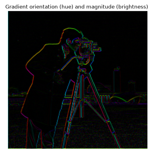
Figure 4a. HSV Gradient orientation map
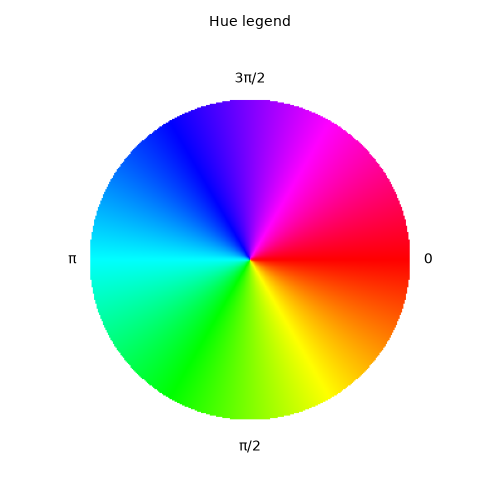
Figure 4b. Hue legend wheel
Orientation Analysis: Vertical edges (like the camera tripod legs) map to Cyan/Blue hues (\(\pi/2\) and \(3\pi/2\)), while horizontal edges (the horizon line) map to Red/Green hues (\(0\) and \(\pi\)). Dark background regions remain black because brightness is scaled by gradient magnitude.